By Joseph Pearson and Jaco du Toit, STANLIB Analytics

Introduction

Investors in active funds expect the portfolio manager to nominate a benchmark, typically a publicly-available index, against which their performance will be judged. The manager’s task is to construct a portfolio which is different from the index to outperform it (though most do not, at least in the equity world).

However, the mandate of passive portfolio managers running ETFs is to replicate the performance of the index as closely as possible. Active managers fear underperformance. What keeps passive managers up at night is tracking error.  An active manager may earn a bonus for beating the benchmark by 5% and a written warning for underperforming by 5%, but an index fund manager gets fired either way.

In simple terms, “tracking error” refers to a single number which describes the difference in the price behaviour a security or portfolio and the price behaviour of a benchmark over a given period of time. Even an ETF that is perfectly indexed will not exactly deliver the performance of its benchmark, even though this difference on a day-to-day, quarter-to-quarter, or year-to-year basis may be minute. Tracking error is the measure of this difference.

In financial markets, no number has meaning without context, and the same applies to the tracking error. The single number allows us to compare the performance of two ETF managers, but it can yield much more insight if broken down into its constituent parts. 

For analysts, “decomposing” tracking error is not merely an esoteric academic pursuit. It reveals the decisions and strategies that shape portfolio outcomes. It provides clarity on where deviations occurred and, crucially, why.

What is tracking error?

Tracking error is precisely what it sounds like: an error or divergence in tracking. Mathematically, it is the standard deviation of excess returns, defined as the difference between the daily return of a portfolio and its benchmark. Conceptually, it describes how consistently a portfolio matches the movements its benchmark. Metaphorically, it is the tyre tracks of a driver in the middle lane of the highway - any more than slight movements to the left or right spell trouble.

There is also a statistical nuance that sometimes goes unremarked. Tracking error describes the variability of excess returns but says nothing about the location of that distribution. A low tracking error per se does not mean that the portfolio will deliver the same return as the benchmark over time.

For example, a fixed income fund benchmarked against three-month JIBAR, which is entirely invested in securities yielding JIBAR +100 bps would outperform by 100 bps with zero tracking error, since the outperformance would be a constant and the standard deviation of a constant is zero.  Many a risk analyst has been asked by an exasperated portfolio manager how their fund could have underperformed by 5% over a year while running a 2% tracking error.  

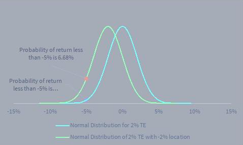
Statisticians will sympathise: a normal distribution around zero with a 2% standard deviation yields a 0.62% probability of a -5% return.

There are two reasons why that scenario could be less unlikely. Firstly, the perfect Gaussian bell-curve of a normal distribution is rarely encountered in real life. The distribution of the excess returns could be non-normal, having skew, kurtosis or fat tails. Secondly, there may be a more mundane reason: the location of the excess return distribution.  As demonstrated in the chart below, if the average excess return is -2% (rather than zero), the statistical probability of 5% underperformance rises by a factor of 10x. 

Figure 1 Tracking Error of excess returns with non-zero location

Source: STANLIB Analytics

But predicting the (future) location of the excess return distribution (i.e. how well the manager will do) is notoriously difficult, because, as the disclaimer in every advertisement for financial products states: “past performance is not indicative of future returns”.

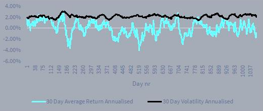
From an ex-ante perspective, we tend to focus on the volatility (i.e. “second moment”) of the excess return distribution. This is because we cling to the belief that while it may not be the case for returns, historic volatility may be a reasonable guide to future volatility. There is some merit to this belief. For example, consider a simulated return of a stock modelled by a normal distribution with an average return of 2% per annum and a volatility of 10% per annum.

Figure 2 Variability of the average return vs the standard deviation of the returns

Source: STANLIB Analytics

Applying a 30-day window to this simulated stock return and calculating an average (first moment) and a standard deviation (second moment) shows significantly less variability in the standard deviation. Because of this lower variability, we focus on tracking error rather than expected excess return. 

Tracking error attribution

If tracking error can provide us with at least some (but not all) information about the future return prospects of the fund relative to the benchmark, which positions in the fund are contributing to this tracking error? The ex-ante tracking error of the fund is given by the equation:

Equation 1

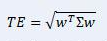
where w is a vector of active weights of positions in the fund vs the benchmark and ∑ is the variance/covariance matrix describing the assets in the portfolio. 

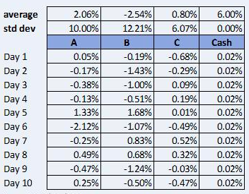
For non-mathematicians, we can also depict this concept without using linear algebra. The following table simulates the daily returns of three securities (A, B and C) and cash on deposit. A fund manager builds a portfolio from these four elements in order to outperform a benchmark in which the three securities are equally-weighted and cash is excluded. 

Figure 3 Simulated Returns

Source: STANLIB Analytics

Figure 4 Portfolio Positioning

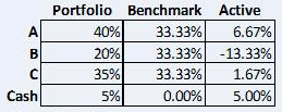
Source: STANLIB Analytics

We can calculate the portfolio’s return relative to the benchmark on any particular day by multiplying each security’s daily return (and that of cash) by its active weight (i.e. the difference between its weighting in the portfolio and its weighting in the benchmark) and then taking the sum of those products for each day in the series. The standard deviation of that sum is the portfolio’s tracking error. It will be identical to the product of the algebraic equation given above.

The above example is based on a daily simulation of the underlying assets’ performance, but to project the tracking error of a portfolio we must rely on the historic volatility of the three securities and their respective correlations.  Since the covariance matrix is obtained from the product of the correlation matrix and the volatility of each asset, we can establish that:

For illustrative purposes, we generated the returns in Figure 3 using an assumed correlation matrix: 

Figure 5 Correlation Matrix

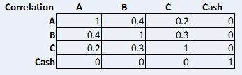
Source: STANLIB Analytics

Assuming that cash is not correlated to any of the assets, and assuming some positive correlation between assets A, B and C as per the correlation matrix above, we can now calculate the volatility and tracking error of the portfolio and the benchmark using Equation 1. We substitute the portfolio weight, benchmark weight or active weights, as appropriate.

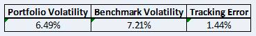
It makes sense that the benchmark is more volatile than the portfolio because it has a heavier weighting to the most volatile asset (B) and has no exposure to cash, which has zero volatility.

We can now calculate the marginal contribution as follows:

1. We first calculate the covariance of each asset to the excess return distribution. In linear algebraic terms this amounts to:

Where w is the active weights and ∑ is the variance/covariance matrix

2. Using this result, we now calculate the correlation of each asset to the excess return distribution:

Where   is the vector previously obtained,   is the volatility vector of each asset and TE is the overall tracking error of the fund.

3. Taking the   vector and multiplying it by the active weight vector   and the volatility vector   gives us the marginal contribution to active risk or MCAR.

For the worked example this results in the following decomposition:

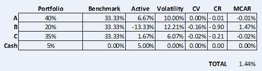
While it makes intuitive sense that security B would be the biggest contributor to the tracking error, because it has the largest active position (i.e. the biggest underweight/overweight versus the benchmark), it is surprising that it effectively accounts for the entire tracking error of the portfolio. Security A is positively correlated to B (0.4) and has similar volatility but half the weighting (20% vs 40%), so it is surprising that A only contributes one basis point to the portfolio’s tracking error.

Notice also that the cash position makes no contribution to tracking error at all. This follows from our mathematical definition of tracking error as the sum of the product of each security’s active weight, correlation and volatility. Since we defined cash as having zero correlation and zero volatility, it follows that its contribution to tracking error must also be zero.

However, it is counter-intuitive for cash to have a zero contribution to tracking error. We can mitigate this by improving on the traditional MCAR methodology by transforming the covariance matrix.

If, instead of using each security’s absolute daily returns, as in Figure 3, we use each security’s daily returns relative to the benchmark, we can construct an active covariance matrix which returns the same overall tracking error for the portfolio (1.44%) but decomposes it in a different way:

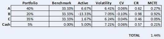
Notice that the score in the volatility column for each of the securities has changed significantly. We are no longer measuring the volatility of each asset’s absolute return, but the volatility of its return relative to the benchmark. This is active volatility, which is synonymous with the tracking error of each security to the benchmark. The CV vector has also changed, as has the CR correlation vector.

The useful output of the original methodology was MCAR (Marginal Contribution to Active Risk). The new approach of using active volatility produces MRCAR (Marginal Relative Contribution to Active Risk). Security B still contributes the most to the tracking error, but is far less dominant, and despite having zero volatility in itself, cash now makes a significant contribution to MCRAR. This makes more sense, since even an asset with a fixed price contributes to the overall tracking error of the portfolio.

MRCAR demonstrates a much closer relationship with the ex-post performance attribution, since the risk contribution of each asset is compared with the benchmark as a whole. This is reminiscent of a Brinson methodology for performance, in which the return of each asset is compared with the return of the benchmark as a whole.

CONCLUSION

Should we use MCAR or MRCAR to best understand how individual assets contribute to the tracking error of a fund? Like so many questions in finance and life in general, the answer is: “it depends”. It is certainly a little harder to estimate the active covariance than the normal covariance matrix. This is because the estimation of each instrument’s excess return requires us to make assumptions about the historic return of the current benchmark (i.e. use the current weights of the benchmark constituents to estimate an historic benchmark return). 

However, the extra work involved in estimating active covariance is more than justified by the greater robustness and real-world character of MRCAR. Some analysts may argue that we have ways of improving the estimation of the normal covariance, such as shrinkage, but those methods can also be applied to the active covariance. 

Complexity aside, we are persuaded that active covariance is the best methodology for decomposing tracking error, taking account of each stock’s tracking error to the benchmark. Employing this approach means that stocks with low volatility or low correlation will not fall by the wayside and allocations to cash will contribute to tracking error as they should. For pure equity funds, this is especially important, as a cash position can drive underperformance in a rising market.